Using Counterfactuals to Understand Machine Learning Models
While machine learning (ML) models have become integral to many drug discovery efforts, most of these models are "black boxes" that don't explain their predictions. There are several reasons we would like to be able to explain a prediction.
- Provide scientific insights that will guide the design of new compounds.
- Instill confidence among team members. As I've said before, a computational chemist only has two jobs; to convince someone to do an experiment and to convince someone not to do an experiment. These jobs are much easier when you can explain the "why" behind a prediction.
- Debugging and improving models. Improving a model is easier if you can understand the rationale behind a prediction.
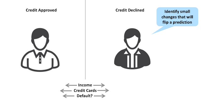
As I wrote in a previous post, identifying and highlighting the molecular features that drive an ML prediction can be difficult. One recent promising approach is the counterfactuals method published by Andrew White's group at the University of Rochester. Counterfactuals have their origins in the assessment of credit risk. In many jurisdictions, a bank must provide an explanation for denying someone credit. The bank can't simply say, "we won't give you a credit card because our neural network doesn't like you". One way of explaining a credit risk prediction is to identify two people with similar characteristics, where one had their credit approved, and another had their credit declined by a black box ML model. The slight differences between these individuals (e.g., the number of credit cards) can then be used to explain the prediction.
We can apply a similar approach to explaining quantitative structure-activity relationships (QSARs). Let's consider an ML model trained to predict aqueous solubility. If we have a molecule predicted to be insoluble, we could gain insights into this prediction by examining predictions for similar molecules predicted to be soluble and noticing where the differences are. For instance, we can generate analogs of Palbociclib, a molecule predicted to be insoluble, and see that replacing a methyl ketone with a carboxylic acid leads to a molecule predicted to be soluble. We can then infer that the methyl ketone may be one cause of poor solubility. As a bonus, we get the structure of an analog predicted to overcome that liability.
Let's take a look at how we would implement something like this. I've assembled a demo Jupyter notebook available on GitHub for those who like code.
1. Generate a set of analogs for a molecule of interest.
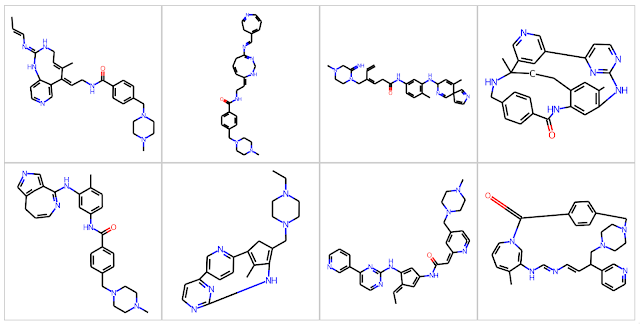
There are several ways to computationally generate analogs for a molecule. In the original publication, Andrew White's group used the STONED SELFIES method to generate a set of analogs. As I pointed out in an earlier post, STONED SELFIES tend to produce a lot of very strange molecules. For instance, if we start with Palbociclib, STONED SELFIES generates these analogs, which I don't find realistic or useful.
The later version of the White group's exmol method uses a reaction-based approach that generates more realistic molecules but sometimes fails to generate a sufficient number of analogs. As an alternative, I used the Chemically Reasonable Mutations (CReM) approach published by Pavel Polishchuk. I wrote a post in 2020 describing how CReM can be used. In short, CReM captures the chemical environments around functional groups and swaps functional groups in similar environments to create new molecules. This is an oversimplification; please check out Pavel's paper for a complete explanation.
2. Generate predictions and similarities for the analogs
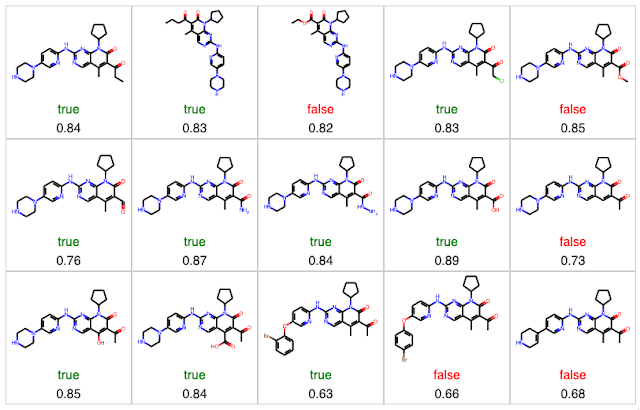
We begin the counterfactual process by generating a set of analogs, calculating their predicted solubility, and their similarity to Palbociclib, our reference molecule. Note that there are a few molecules in the set below that I should have eliminated using functional group filters.
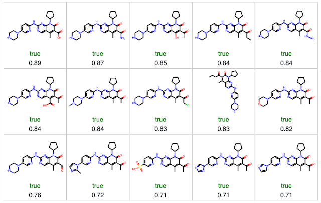
Since Palbociclib is predicted to be insoluble (labeled as false), we want to examine similar molecules predicted to be soluble (labeled as true). We can do this by selecting only the molecules where the prediction is "true" and sorting by similarity.
4. Examine detailed comparisons
To simplify comparisons, I added a routine that will align pairs of molecules and highlight their differences. For more on this, please check out the code.
Counterfactuals provide an intuitive understanding of machine learning predictions and can suggest ways to overcome liabilities. Please give the code a spin and see if you find it helpful. Andrew White's group has an excellent Perspective article in JCTC that describes counterfactuals and several other approaches to explainable ML for molecules.


Fascinating article and thanks for such a clear explanantion of this topic. I love your blog! While in the Chemoinformatics QSAR world, using Counterfactual is a cool new way to analyse 'black box' ML models and I believe has parallels to the traditional 'open box' Matched Pair Analysis, the broader connections between Causal Inference methodologies and ML methodologies is becoming ever deeper.
ReplyDeleteHere as you so well put it, Causal Inference is being used to explain ML QSAR models; there are scanarios where ML models are being made more "transportable" using Causal Inference methodologies and even more interestingly ML models are enhacing Causal Inference itself by providing "valid" counterfactual inferences. These ideas are coming out from Epidemiology and Econometrics fields.
Just on nomenclature, aren't these "activity cliffs", but for predicted properties? I like the idea of retaining that nomenclature to link it to the existing literature.
ReplyDeleteThanks, Noel. I don't know if "activity cliffs" are exactly what we're talking about here. In this case, we're referring to a structural change that flips the label from one category to the other. That change doesn't necessarily have to be huge. In the case of activity cliffs, we have a small change in chemical structure that leads to a large change in an activity or property. I see a subtle distinction, but others may disagree.
Delete