Comparing Classification Models - You’re Probably Doing It Wrong

In my last post, I discussed benchmark datasets for machine learning (ML) in drug discovery and several flaws in widely used datasets.  In this installment, I’d like to focus on how methods are compared.  Every year, dozens, if not hundreds, of papers present comparisons of ML methods or molecular representations.  These papers typically conclude that one approach is superior to several others for a specific task.  Unfortunately, in most cases, the conclusions presented in these papers are not supported by any statistical analysis. I thought providing an example demonstrating some common mistakes and recommending a few best practices would be helpful.  In this post, I’ll focus on classification models.  In a subsequent post, I’ll present a similar example comparing regression models.  The Jupyter notebook accompanying this post provides all the code for the examples and plots below.  If you’re interested in the short version, check out the Jupyter notebook. If you want to know what’s going on under the hood, please read on.

An Example

As an example, we’ll use the dataset presented in a recent paper by Diwan, AbdulHameed, Liu, and Wallqvist in ACS Omega.  In this paper, the authors used a few different ML approaches to build models for bile salt export pump (BSEP) inhibition. They concluded that multi-task machine learning provides a superior model.  To reproduce the published work, I built machine learning models using the dataset the authors provided in their GitHub repository.  In the example presented below, I compared three different ML approaches. 

• LightGBM (LGBM) with RDKit Morgan fingerprints and a path length of 2, sometimes called ECFP4.  This is the “conventional ML” baseline. 
• A single task message passing neural network (MPNN) as implemented in ChemProp (CP_ST). This provides an example of single-task deep learning. 
• A multi-task MPNN as implemented in ChemProp (CP_MT), which acts as the multi-task deep learning method. 

I performed 10 folds of cross-validation where all models were trained on the same cross-validation splits.  I did two sets of comparisons, one using a random split and the other using a scaffold split. Note that I used a relatively simple cross-validation strategy here.  For more sophisticated approaches, please see this post.  The code used to build the models, and the results from the cross-validation folds are available in the GitHub repository associated with this post.  To evaluate the performance of the models, I applied three widely used performance metrics. 

• Area Under the Receiver Operating Characteristic (ROC AUC)
• Area Under the Precision-Recall Curve (PR AUC) 
• Matthews Correlation Coefficient (MCC)

There are differing degrees of religious fervor around which metrics are most important.  In the interest of completeness, I’ve included all three. 

The (Wrong) Way Methods are Typically Compared 

Most papers in our field present the comparisons of classification models in one of two ways.  The first is what I refer to as “the dreaded bold table”.   Many authors simply report a table showing the average for each metric over N-folds of cross-validation.   The method with the highest value for a particular metric is shown in bold.  <sarcasm> The table below shows us that the multi-task ChemProp (CP_MT) model outperforms the other two models because it’s the “winner” on two of three metrics, right?  </sarcasm>

The other common approach to comparing classification models is to present a “dynamite plot” showing the mean metric value for the cross-validation folds as a bar plot with error bars showing the standard deviation over the cross-validation folds.  Papers rarely discuss the standard deviation or the significance of the differences between the cross-validation averages. 

Why Is This Wrong? 

When comparing metrics calculated from cross-validation folds for an ML model, we’re comparing distributions.  When we compare distributions, we need to look at more than just the mean.  If we look at the two distributions below, it seems intuitively obvious that the distributions on the left are different, while the distributions on the right are similar. 

A common way of determining whether two distributions are different is to look at the overlap of the error bars in a dynamite plot, like the one shown in the previous section.  Unfortunately, this approach is incorrect. It’s important to remember that the standard deviation is not a statistical test. It’s a measure of variability.  The "rule" that non-overlapping error bars mean that the difference is statistically significant is a myth. This rule doesn't apply to any conventional type of error bar.  For a detailed discussion of the incorrect “non-overlap of error bars” rule, see this paper by Anthony Nicholls. 

Statistical Comparisons of Distributions 

Fortunately, statisticians have spent the last 150 years developing tests to determine whether the arithmetic means of two distributions differ.  The most widely known of these tests is Student’s t-test, which we can use to compare the means of two distributions and estimate the probability that the difference could have arisen through random chance.  One output of the t-test is a p-value, which indicates this probability.  Typically, a p-value less than 0.05, indicating a random probability of less than 5%, is considered significant.  While the t-test is an essential tool, it has some limitations.  First, the distributions being compared should be normally distributed.  When we deal with a small number of folds from cross-validation, it’s difficult to determine that our calculated metrics are normally distributed.  Second, the distributions need to be independent.  While the training and test sets are independent over a single cross-validation fold, samples are reused over subsequent folds.  Third, the distributions should have equal variance.  Some have argued that the magnitude of this variance is diminished over cross-validation folds.  

An alternative approach that overcomes these limitations is to use a non-parametric statistical test.  Non-parametric tests, which typically operate on rank orders rather than the values themselves, tend to be less powerful than analogous parametric tests but have fewer limitations on their application.  Most parametric statistical tests have non-parametric equivalents.  For instance, the Wilcoxon Rank Sum test is the non-parametric analog for Student’s t-test.  

This all sounds great, but I tend to learn from examples.  Let’s compare ROC AUC from the three methods listed above on the BSEP dataset.  We’ll start by comparing pairs of methods.

• CP_ST vs LGBM
• CP_MT vs LGBM
• CP_MT vs CP_ST

The plots below compare the distributions of ROC AUC for the method pairs.  Above each plot, we have the p-values from Student's t-test and the Wilcoxon rank sum test.  Examining the figure on the left, which compares the single-task and multitask ChemProp AUCs, we see the two distributions overlap, and the p-values from the parametric and non-parametric tests are nowhere near the cutoff of 0.05.  One would be hard-pressed to say that multi-task learning outperforms single-task learning in this case.  In the center plot, we see a clear difference between the distributions, and both the parametric and non-parametric p-values are below 0.05.  In the plot on the right, the parametric p-value is slightly over 0.05, and the non-parametric value is slightly below.  

While plotting the kernel density estimates as we did above is informative, I prefer to look at this sort of data as boxplots.  The plots below show the distributions above as boxplots.  For me, this provides a clearer view of the differences in the distributions. The boxplots make it easier to see the distribution median, where most of the data lies, and where the outliers are. 

Comparing More Than Two Distributions

There’s another aspect we need to consider when comparing the above distributions.  The statistical tests we’ve discussed so far are designed to compare two distributions.  As we add more methods, the chances of one method randomly being better than another increases. The ANOVA, or analysis of variance, provides a means of comparing more than two methods.  While the ANOVA is a powerful technique, it suffers from some of the same limitations as the other parametric statistical methods described above.  Friedman’s test, a non-parametric alternative to the ANOVA, can be used in cases where the data is not independent or normally distributed.  Friedman’s test begins by reducing the data to rank orders.  In this example, we will consider the same comparison of AUC for 3 methods.  We start by rank-ordering the methods across 10 folds of cross-validation.  In the figure below, each row represents a cross-validation fold, and each column represents a method.  A cursory examination shows that multi-task ChemProp (CP_MT) was ranked first 4 times, single-task ChemProp (CP_ST) was ranked first 5 times, and LightGBM (LGBM) was ranked first only once. 

We then calculate the rank sums for each column and see that ChemProp single-task has the lowest rank sum. 

The values from this analysis can then be plugged into the formula below to calculate the Friedman χ2.

Where N is the number of cross-validation folds, k is the number of methods, and R is the rank sums. 

I don’t typically think in terms of χ2 values.  To develop some intuition for this, I plotted χ2 vs p. 

It's trivial to convert χ2 to a p-value using scipy.  

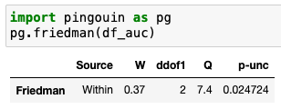
Of course, we don’t have to jump through these hoops to perform Friedman’s test.  There are implementations in pingouin, scipy, and several other Python libraries.  Here’s an example with pingouin.

Here’s the same example with scipy (and far too many decimal places). 

Using Friedman’s Test to Compare Models of the BSEP Dataset

Now that we have the preliminaries out of the way.  Let’s apply Friedman’s test to the BSEP dataset we discussed above.  The figure below shows one way I like to compare methods.  The code used to generate this figure is in the Jupyter notebook associated with this post.  Boxplots show comparisons of the three methods with ROC AUC, PR AUC, and MCC over 10 cross-validation folds.  Above each plot, we have the p-value from Friedman’s test.  In this example we randomly split the data into training and test sets.  While we see a significant p-value for ROC AUC, the p-values for PR AUC and MCC are not significant.  Is one method superior to another?  Given this analysis, it’s hard to say.  

If we look at the results below, where we used scaffold splits for cross-validation,  we see a similar trend.  There is a statistically significant p-value from Friedman’s test for ROC AUC, but the p-values for PR AUC and MCC are not significant. 

Post-hoc Tests

At this point, the astute reader may have noticed that Friedman’s test tells us if a difference exists between methods but doesn’t tell us where this difference is.  Once we’ve used Friedman’s test to confirm a difference between methods, we can use a post-hoc test to determine where the differences are.  Post-hoc tests are just pairwise statistical tests of the individual methods, with one crucial difference.  As mentioned above, when we compare more than two methods, there is a higher likelihood of one method being better by chance.  To deal with this, we typically correct the threshold p-value for significance.  One of the most straightforward approaches to adjusting the threshold for significance is the Bonferroni correction.  With this correction, the threshold for significance is divided by n, where n is the number of methods being compared.  For instance, if our threshold for significance is 0.05 and we are comparing 3 methods, the threshold becomes 0.05/3 or 0.017.  Some argue this is too harsh, and several alternatives have been proposed.  You might be thinking, “If we have post-hoc tests, why do we need to perform Friedman’s test?”.  Remember that post-hoc tests compare pairs of methods, while Friedman’s test compares all.  It’s crucial to perform both tests.

Let’s take a look at an example. In the plots below, we use the pairwise Conover-Friedman test implemented in the scikit-posthocs package to perform the post-hoc tests.  In the interest of brevity, we’ll only consider the scaffold split example. In these “sign plots”, each cell shows the significance of the corrected p-value representing the difference between the two methods indicated in the rows and columns.  The diagonals, which represent a comparison of the method with itself, are white.  The color in the cells represents the degree of statistical significance. The corrected p-values greater than 0.05 (NS = not significant) are colored pink.  Significant p-values are shown in progressively darker shades of green.    As expected based on Friedman’s test, we see a difference between LGBM and the other methods for ROC AUC.  None of the other comparisons was significant. 

Another tool for comparing multiple methods is the Critical Difference Diagram (CDD), which is also available in scikit-posthocs.  In the CDD, if two methods are connected by a horizontal line, there is no significant difference between the distributions.  The position of a vertical line in the CDD represents the mean rank of a method over cross-validation folds.  In the top plot in the figure below, we have a CDD for ROC AUC.  This plot shows that LGBM has a low mean rank of 0.4, and there is no horizontal line between LGBM and the other two methods.  This indicates the difference between LGBM and the two ChemProp variants is significant.  For CP_ST and CP_MT, we see similar average ranks and a horizontal line between the vertical lines, indicating that the difference between methods is not significant.  In the two lower plots, we see a black horizontal line connecting all three vertical lines.  This indicates that there is not a significant difference between methods.  As with the analysis above, it’s tough to say that any of the three methods outperforms the others. 

Conclusions

I realize the title of this post is provocative and may have come across as arrogant.  I'm not the ultimate expert on statistics, and there may be better ways of comparing methods than what I've outlined here.  However, we need to do something to improve the state of our field, and we need to do it now.  Most papers published today use highly flawed datasets and completely ignore statistical analyses.  This needs to stop.  I think the best way to change the current situation is to provide clear guidelines on best practices.  These guidelines can then be adopted by authors, reviewers, and editors.  I’m working with a few friends to assemble a first draft, which we hope to publish as a preprint before the end of this year.  If you’d like to help, please let me know.