Multiple Comparisons, Non-Parametric Statistics, and Post-Hoc Tests

In Cheminformatics, we frequently run into situations where we want to compare more than two datasets.  When comparing multiple datasets, we have a higher probability of chance correlation so we must make a few adjustments to the ways in which we compare our data.  In this post, we will examine the impact of multiple comparisons and talk about methods known as post-hoc tests that can be used to correct p-values when multiple comparisons are performed.  We will also make a brief foray into non-parametric statistics, a technique that is appropriate for dealing with the skewed data distributions that we often encounter in drug discovery.  As usual, all of the data and the code used to perform the analyses in this post is available on GitHub.  

I always find it easier to understand a method when I’m presented with an example.  For this case, we’ll look at a 2011 paper from Li and coworkers.  In this paper, the authors compared the impact of nine different charge assignment methods on the performance of the docking program Autodock 4.2.  The study was relatively straightforward.  The authors used each of nine different methods to assign atomic partial charges to a set of ligands.  They then looked at the impact of the charge assignment method on the ability of the docking program to reproduce the crystallographic pose.   The resulting data is a table of RMS fit values (smaller is better) for each protein-ligand complex/charge assignment combination.  To provide some context, here the first few lines of the data table. 

Once the data had been collected, the authors calculated the mean RMS fit for each of the charge assignment methods and determined that Gasteiger-Huckel and AM1-BCC charges produced the best results (hmm).  Let’s take a look at this data and see if we agree with the conclusions from this paper.   We’ll start out by doing something close to what was done in the paper.  We’ll plot the mean values along with error bars showing the standard deviations.  

As we can see from the plots above, Gasteiger-Huckel does indeed have a low RMSD but look at the error bars.  It seems like there is quite a bit of overlap.  In addition, the plot above is just a variant on the infamous dynamite plot.  If you read my last post, you’ll know that there are better ways to look at distributions.  Let’s look at the same data as a boxplot.  

Based on the boxplots above, we can see that there is quite a bit of overlap in the distributions.  This indicates that there probably isn’t a clear winner, but we’d like to know if there is a statistically significant difference in the mean values for the nine reported distributions. As many of us remember from our undergraduate Analytical Chemistry class, we can use a t-test to compare the means of two distributions.  The thing that Chemistry professor failed to mention (at least mine did) is that the t-test is only applicable when certain conditions are met. 

• The data is normally distributed
• The data is drawn from independent distributions
• The variance within the groups is equal within the population

The first condition is rarely met in drug discovery.  We often deal with distributions that are skewed, bimodal, or just hard to describe.  It’s often easy enough to just visualize the distribution and determine whether it’s normal.  We can do that with the data from this paper.  Looking at the figure below, we can see that the distributions don't appear to be normal. 

There are also statistical tests such as the Shapiro-Wilk test that can be used to get a more quantitative description of the normality of a distribution.   In the Shapiro-Wilk test, the null hypothesis is that the data is normally distributed, thus a p-value less than a chosen alpha (typically 0.05) indicates that the data is not normally distributed.  If we calculate a p-value for our datasets with the Shapiro-Wilk test, we can see that none of the distributions is normal. 

For more on statistical tests for normality and associated Python code, see this page by Jason Brownlee.  If you’re interested in applications of statistics and machine learning in Python, check out Brownlee's books they’re all great! 

Let’s consider the second factor, “the data is drawn from independent distributions”, what does this mean?  Let’s consider a classical clinical trial, where we have a treatment group and a control group.  The treatment group is completely independent of the control group, there is no overlap of patients between the groups.  Now let’s consider the case like the one above where we are comparing the impact of different approaches for charge assignment on the performance of a docking program.  In this case, each charge assignment method is applied to every molecule in the dataset.  The same samples are used for every method, so the samples are not independent. 

We’ve already violated two of the necessary conditions for applying the t-test, so it’s time to look for another method.  Fortunately, we can rely on a field known as non-parametric statistics. Rather than dealing directly with the values in our data table, non-parametric statistics typically deals with the rank orders of the values.  There are a number of non-parametric tests for comparing distributions, but one of the most commonly employed is the Mann Whitney U test.  This post is getting kind of long so I won’t go into a lot of detail on how the Mann Whitney test works.  If you’re interested in the inner workings of this test, check out the corresponding Wikipedia Page.  

While a non-parametric test like Mann-Whitney can be used with a non-normal distribution, we can’t use the p-values obtained by comparing pairs of distributions to directly compare the significance of the difference in the means when more than two methods are compared. 

As an example, let’s assume we’re conducting a clinical trial of a blood pressure lowering agent, and that our null hypothesis is that the means of the distributions of responses for the treatment and control groups are equal.  Let’s further assume that in order to compare the mean values for our control and treatment groups, we perform a t-test and obtain a p-value of 0.05.  This p-value indicates that there is a 5% probability that our result could have occurred by chance.  Of course, this is for two tests.  If we had performed 3 tests, our chance of randomly invalidating the null hypothesis would be 3 * 5% or 15%.  

A number of corrections for multiple testing have been developed.  One of the simplest is the Bonferroni correction where the alpha value required for significance is divided by the number of tests being performed.  So if we are performing 3 tests and we use 5% as our threshold for significance (p=0.05) we would need a p-value of 0.05/3 or 0.017 in order to conclude that the difference in the mean values is significant. The Bonferroni correction works well when 3 or 4 comparisons are considered, but becomes overly conservative when the number of comparisons becomes large.  An alternate, and preferred, technique is known as Holm’s method.  In Holm’s method, the correction factor is adjusted downward as the number of tests becomes larger.  This adjustment allows Holm’s method to avoid the tendency of the Bonferroni correction to become overly conservative as the number of tests increases. 

Fortunately, if we’re programming in Python, we don’t have to worry too much about the mechanics of correcting for multiple comparisons.  There is a well written and easily installed package, called scikit-posthocs,  to do the work for us.  Maksim Terpilowski, the author of this package, has implemented a number of methods to perform statistical tests when multiple comparisons are being made.  In addition, the package displays a helpful graphic to aid in the interpretation of the results.   In this graphic, all of the adjusted pairwise p-values are shown as a heatmap where significant p-values are colored green and non-significant p-values are colored red.  Let’s take a look at our dataset using this repesentation. 

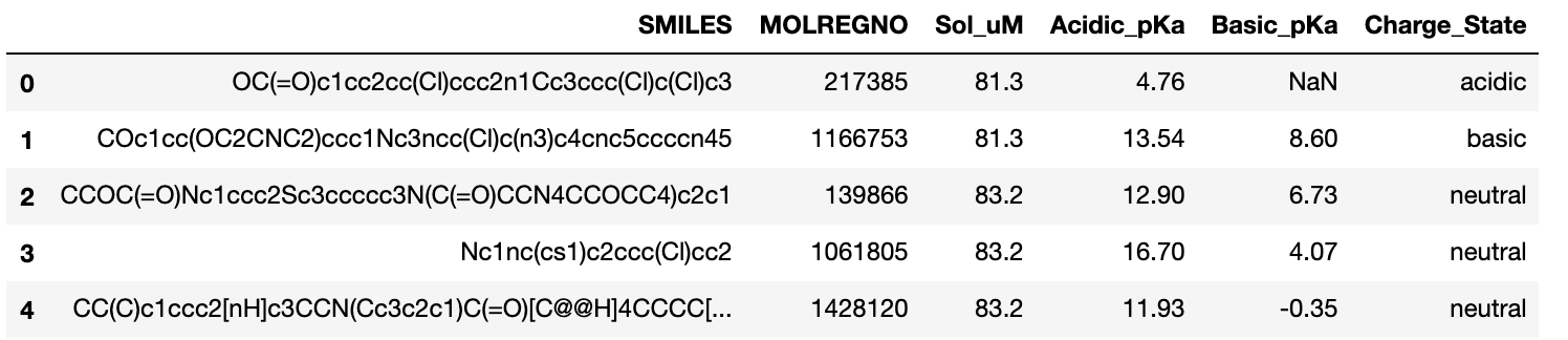
It turns out that none of the differences is significant. That’s kind of a bummer and it doesn’t really show the power of scikit-posthocs.  Let’s take a quick look at one more example.  In this case, we’ll use a dataset that I’m using for a talk at the 2019 ACS National Meeting in Orlando.  The ACS talk, entitled “The Utility of Acidic and Basic Compounds in Medicinal Chemistry” is a follow-on to a paper that Paul Charifson and I published in J. Med. Chem in 2014.   The talk (and the paper) are focused on the different behaviors of acidic, basic, neutral and zwitterionic compounds, and how these properties can be used in drug discovery. For the purposes of this example, we’ll look at a set of 1,763 compounds with measured solubility from the ChEMBL database.  I calculated the major microspecies for each of these molecules and classified them as acidic, basic, neutral, or zwitterionic. The first few rows in the table look like this.



The critical columns in the table are "Sol_uM" the thermodynamic solubility in uM and "Charge_State" which indicates whether the compound is acidic, basic, neutral, or zwitterionic at pH 7.4.  Let's look at the data as a boxplot.  We can see that neutral compounds are less soluble than charged compounds. It also looks like there's some difference between acidic and basic compounds.

Let's use scikit-posthocs to see if any of these differences are significant. If we look at the first row in the table below, we can see that there is a significant difference between the solubility of acidic and basic compounds (p < 0.05). The difference between acidic and neutral compounds is more significant (p < 0.001). However, the difference in the mean solubilities of the acidic and zwitterionic compounds is not significant. We can look across subsequent columns to examine the differences between basic, neutral, and zwitterionic compounds.

This post is already really long so I should probably bring this one to a close.  Hopefully, I've shown you that there's quite a bit that needs to be done to properly compare computational methods.  While there's a lot to this, packages like scikit-posthocs make it easy to do the comparisons.  The next time you publish or review a paper, remember to consider the impact of multiple comparisons.  Please checik out the code on GitHub.